Non-Parametric Bootstrap Model
Motivation
The next prediction method we used is derived from "A Simulation-Based Model for Final Price Prediction in Online Auctions" by Chou et al. In this paper, the prediction method calls for simulating the progression of an auction. Given a starting price and auction length, they sample (time increment, bid increment) from the empirical distribution from past auctions. They repeatedly sample from this empirical distribution, adding on to previous samples, until the total time exceeds the length of the auction. The total price at this time is this simulation's prediction of the end price, and they average over many simulations to get a final price prediction for the auction.
Chou et al. used this method to predict final prices in Yahoo! camera auctions. In our setting, final prices in eBay car auctions have too much variation for this method to work well on its own. Car values depend heavily on make, year, and mileage, but their method lumps together extremely dissimilar cars, such as cars with 500,000 miles and brand-new cars with 0 miles. In our test set, the average prediction error for the unconditional bootstrap is 183%. Thus, it performs worse than both baseline methods.
To overcome the issue of including very dissimilar cars in our empirical distribution, we limit the empirical distribution to a subset with similar features to the auction that we are trying to predict. One method involves taking the subset where cars have mileages, years, and starting prices in the same quintile as the car whose price is being predicted, as well as the same model. Other methods involve only using mileage quintiles, only year quintiles, only starting price quintiles, only the model, only the brand, or some combination thereof.
Implementation
Goal: Predict the final price of the auction given features provided at the start of the auction, including mileage, year, starting price, model, and brand
1. Split the data into training and test sets
2. For each auction in the test set, find the restricted empirical distribution of (time increment, bid increment) based on that auction's features
3. Draw from this empirical distribution to simulate an auction
4. For each auction in the test set, run 100 simulations and take their average as our prediction
Results
Below are graphs illustrating the results of our representative bootstrap method, which involves mileage and year quintiles, as well as subsetting on brand. The average error was 152%, with a standard deviation of 6.40%.
| Predicted and True Prices | Differences |
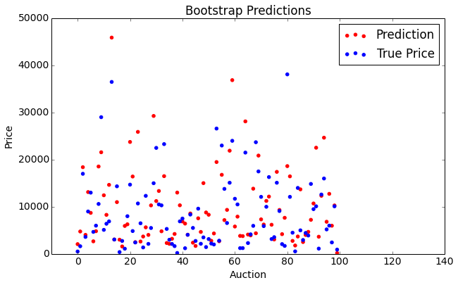 | 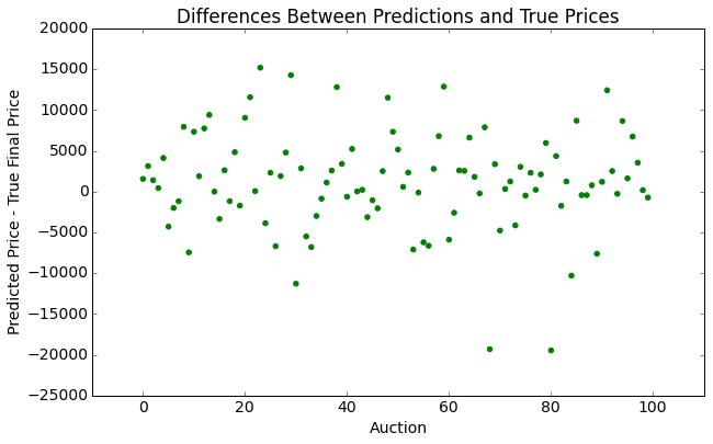 |
Analysis
Why does this model result in such large errors? The graph below on the left suggests that it performs particularly poorly for auctions with final prices of less than $2000. In fact, the average error for auctions less than $2000 is 669%, while the average error for auctions greater than $2000 is 54%. The graph below on the right suggests a reason the bootstrap method performs so poorly for auctions with final prices under 2000. It shows that many of these supposed cars have mileages of 0, which implies that they are brand-new cars. It is highly unlikely for a brand-new car to be sold on eBay for less than 2000, so the true reason behind these 0 mileages is probably that these items are not actually cars. Items are occasionally miscategorized on eBay, so the presence of items that are not actual cars may skew our predictions if (time increment, bid increment) distributions inherently differ based on the item.
| Final Price Comparison | Differences |
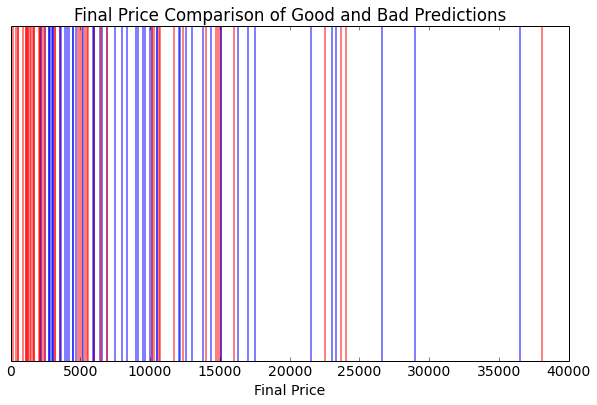 | 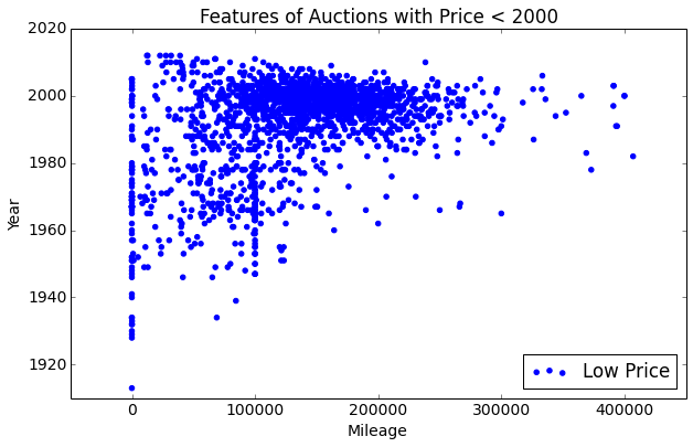 |
Dropping observations for which the mileage is 0 and the final price is less than $10,000 reduces the average error of the bootstrap method to 119%, demonstrating the importance of data accuracy. Further identifying items that are not actually cars may additionally reduce prediction error.