3-Factor Price Velocity Acceleration Model
Motivation
For my model on price prediction for ebay auction time series data, I drew inspiration from the paper title "Modeling Price Dynamics in eBay Auctions Using Principal Differential Analysis" by Wang et al. After reading that paper, what really struck me as interesting was the idea of velocity and acceleration with respect to prices. I found that idea to be very power, and I decided to use this idea to attempt to create a model for price prediction based on velocity and acceleration of prices.
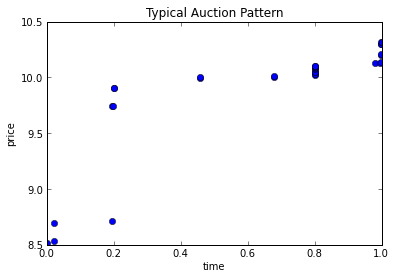
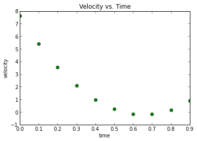
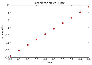
Before beginning my analysis, let me run down a quick intuition behind my model. As stated in Wang et al.'s paper, human psychology tends to the drive the behavior of bidding in online auction markets such as ebay, and the following phenomenon is often observed: we start off at the initial points of the auction with some fairly rapid bidding, where the price increases from starting value to a reasonable value, following this period is a lengthy time of little to no bitting as consumers want to hide their valuation of the item until the last second, and just before the end time of the auction, we see extremely rapid bidding, shooting the price to its final value. In accordance with the described price movement, velocity (first derivative of the price curve) will begin postive, curve downwards towards zero before shooting back up to positive again. Acceleration (2nd derivative of the price curve) on the other hand, begins negative, crosses zero and becomes hugely positive towards the end of the auction.
Below is a visualization of the typical trends observed in an auction:
| Price Levels | Velocity |
 |  |
| Acceleration | |
 |
Thus, in an attempt to model this type of behavior, I decided that the velocity of bidding and the acceleration of prices are the most influential factors deciding an auction's final price.
Implementation
Goal: Predict the final price of the auction given 90% of the time series bidding data through a 3 factor linear model based on price, velocity, and acceleration
1. Split the data into 90% and 75% of the time series
2. Fit a cubic polynomial curve to 90% and 75% of the data, respectively and calculate the 1st and 2nd derivatives of each model
3. Use 75% of the data to train the 3 factor model and determine the estimated weights of each factor
Create a system of equations in the form Ax = B, where A is a matrix of price,velocity, and acceleration values
, and B is a matrix of price levels at a certain time point
Backsolving for x will determine the weights of the 3 factors
These equations will come from iteration of the training set from 75% of the data to 90% of the data, creating one equation for each data point in that interval
4. Use the weights estimated in the previous step as well as price, velocity, and acceleration estimates in the last time step of 90% of the data to predict the final price
Results
Below is a visualization of a sample prediction as well as the % error after running the model on ~25,000 completed auctions
| Sample Prediction | Percent Error |
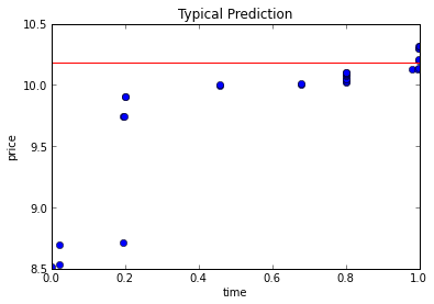 | 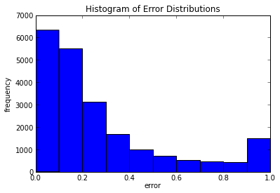 |
The median error is around 17% with standard deviation of 27%
Analysis
Although the model makes pretty solid predictions, its results should be taken with the following discretions
1. Only auctions that had 20 or more bids were considered in this algorithm, and thus its results cannot be generalized to small bid number auctions
2. We discarded around 20% of results, that exhibit extreme errors due to instability of the weighting algorithm that sometimes created extreme weights that produced very large errors
Further work related to this model and/or line of thought include:
1. Creating and implementing a more stable weight selection algorithm, potentially based on matching auction curves for the prediction with similar curve shapes in training set
2. Attempting other functional fitting of original price data such as spline interpolation or nonlinear/piecewise functions